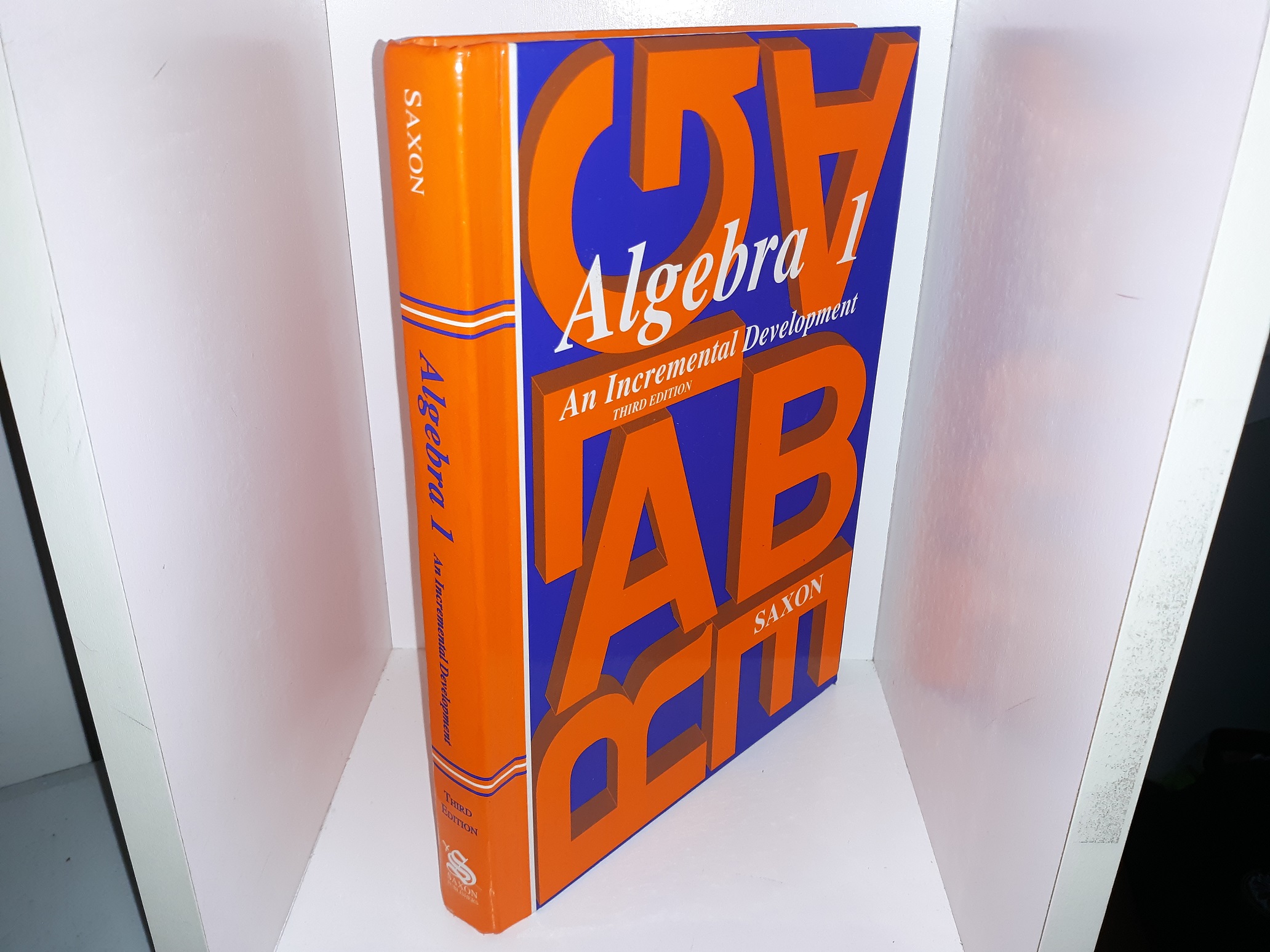
Algebra 1 an incremental development – Algebra 1: An Incremental Development for Success is a journey of unlocking the power of mathematical thinking, one step at a time. This approach transforms the learning process from a daunting task into a rewarding adventure, empowering students to grasp the intricacies of algebra with confidence and ease.
By breaking down complex concepts into smaller, manageable pieces, incremental development allows students to build a strong foundation, gradually expanding their understanding as they master each component. This approach fosters a deeper comprehension of algebraic principles, paving the way for success in higher-level mathematics and beyond.
Introduction to Algebra 1

Algebra 1 is a fundamental branch of mathematics that lays the groundwork for higher-level mathematical concepts and applications. It introduces the core principles of variables, expressions, equations, and inequalities, providing the tools to solve a wide range of problems in various fields. Understanding these concepts is crucial for success in science, engineering, economics, and many other disciplines.
Variables
Variables are symbols that represent unknown quantities or values that can change. They are typically represented by letters, such as x, y, or z. For example, in the equation “x + 2 = 5”, the variable “x” represents the unknown value that, when added to 2, equals 5. Variables can be assigned different values depending on the context of the problem.
Expressions
Algebraic expressions are combinations of variables, constants, and mathematical operations. They represent a mathematical statement that can be evaluated to obtain a numerical value. Examples of expressions include:
- 2x + 3: This is a binomial expression consisting of two terms, 2x and 3.
- 5x²
-2x + 1: This is a trinomial expression consisting of three terms. - 4y: This is a monomial expression consisting of one term.
Expressions can be simplified by combining like terms and applying the order of operations. Evaluating an expression involves substituting specific values for the variables and performing the operations to obtain a numerical result.
Equations
Equations are mathematical statements that express equality between two expressions. They typically have a left-hand side (LHS) and a right-hand side (RHS) separated by an equal sign (=). The goal of solving an equation is to find the value(s) of the unknown variable(s) that make the equation true.
- Linear equations: These equations have a variable raised to the power of 1. For example, 2x + 3 = 7.
- Quadratic equations: These equations have a variable raised to the power of 2. For example, x² + 2x – 3 = 0.
Solving equations involves using algebraic operations to isolate the variable on one side of the equation.
Inequalities
Inequalities are mathematical statements that express a relationship between two expressions, where one expression is either greater than, less than, greater than or equal to, or less than or equal to the other expression. They are similar to equations but use inequality symbols ( <, >, ≤, ≥) instead of an equal sign.
- Linear inequalities: These inequalities have a variable raised to the power of 1. For example, 2x + 3 < 7.
- Quadratic inequalities: These inequalities have a variable raised to the power of 2. For example, x² + 2x – 3 > 0.
Solving inequalities involves finding the range of values for the variable that satisfy the inequality. The solutions are typically represented graphically on a number line.
Real-World Applications
Algebra 1 concepts are widely applied in real-world scenarios, helping us understand and solve problems in various fields. Here are some examples:| Scenario | Concept | Explanation ||—|—|—|| Calculating the cost of a phone plan based on the number of minutes used | Linear equations | The cost of the plan can be represented by a linear equation, where the variable represents the number of minutes used.
Solving the equation allows us to determine the total cost. || Determining the area of a rectangular garden | Quadratic equations | The area of a rectangle is calculated by multiplying its length and width. If the dimensions are expressed as variables, the area can be represented by a quadratic equation. Solving the equation allows us to find the area of the garden.
|| Calculating the speed of a car | Linear equations | The speed of a car can be calculated by dividing the distance traveled by the time taken. If the distance and time are expressed as variables, the speed can be represented by a linear equation. Solving the equation allows us to determine the car’s speed. || Comparing the cost of two different loan options | Inequalities | The cost of a loan can be represented by an inequality, where the variable represents the interest rate.
Solving the inequality allows us to determine which loan option is more affordable. || Determining the optimal production level for a company | Quadratic equations | The profit of a company can be represented by a quadratic equation, where the variable represents the production level. Solving the equation allows us to find the optimal production level that maximizes profit. |
Importance of Algebra 1
Algebra 1 serves as a fundamental building block for higher-level mathematics, providing the necessary tools and concepts for understanding more complex mathematical ideas. The skills and knowledge gained through learning Algebra 1 are essential for success in various fields, including:
- Science: Algebra 1 is used extensively in physics, chemistry, and biology to model and solve problems related to motion, chemical reactions, and biological processes.
- Engineering: Engineers use Algebra 1 concepts to design structures, analyze systems, and solve complex problems related to mechanics, electronics, and other engineering disciplines.
- Economics: Economists use Algebra 1 to model economic systems, analyze data, and make predictions about economic trends.
Incremental Development in Algebra 1
Imagine you’re trying to climb a mountain. It’s much easier to reach the summit if you break the journey down into smaller, manageable steps, right? Learning Algebra 1 is similar! Incremental development helps you break down complex concepts into smaller, easier-to-understand pieces. This makes the learning process less overwhelming and more enjoyable.
Benefits of Incremental Development
Incremental development in Algebra 1 allows you to build a strong foundation of knowledge, step by step. It’s like building a house – you start with the foundation, then add the walls, roof, and so on. Each step is essential, and they all work together to create a solid structure.
Building Deeper Understanding
- Start with the basics: Before tackling complex equations, incremental development ensures you master the fundamental concepts of variables, expressions, and operations.
- Connect concepts: Each new concept builds upon previous knowledge, creating a strong network of understanding. For example, understanding linear equations is crucial for later learning about quadratic equations.
- Develop problem-solving skills: Incremental development encourages you to break down complex problems into smaller, more manageable steps. This improves your problem-solving skills, making you a more confident and capable learner.
The Power of Practice and Repetition
Practice is the key to mastering any skill, and Algebra 1 is no exception. Incremental development emphasizes regular practice and repetition. By consistently working through examples and exercises, you solidify your understanding of each concept. Think of it like playing a musical instrument – the more you practice, the better you become!
Implementing Incremental Development
| Step | Description |
|---|---|
| 1. Define Learning Objectives | Clearly identify the specific concepts and skills to be taught in each lesson or unit. |
| 2. Break Down Concepts | Divide complex topics into smaller, manageable chunks. |
| 3. Provide Clear Explanations and Examples | Use a variety of teaching methods to ensure understanding. |
| 4. Incorporate Practice and Feedback | Offer regular opportunities for students to practice and receive feedback. |
| 5. Review and Reinforce | Regularly review previously learned concepts to solidify understanding. |
A Story of Success
Sarah was struggling with Algebra 1. She felt overwhelmed by the complex equations and abstract concepts. Her teacher introduced an incremental development approach, breaking down the material into smaller, more manageable steps. Sarah started with the basics, mastering each concept before moving on to the next. She practiced regularly and received feedback from her teacher and classmates.
As Sarah progressed, she felt a sense of accomplishment and confidence. She began to see the connections between different concepts, making Algebra 1 more engaging and rewarding. Sarah’s journey is a testament to the power of incremental development in overcoming challenges and achieving success in Algebra 1.
Building Blocks of Algebra 1
Algebra 1 is like building a magnificent tower. Each concept is a brick, carefully placed, contributing to the overall structure. Understanding these building blocks is crucial for mastering Algebra 1 and unlocking its power to solve real-world problems.
Fundamental Concepts
These are the foundational bricks that form the base of the tower. Without a solid foundation, the tower cannot stand.
- Numbers and Variables: The building blocks of Algebra 1 are numbers and variables. Numbers represent specific quantities, while variables represent unknown values. We use variables to represent quantities that can change, like the number of apples in a basket or the speed of a car. For example, “x” could represent the number of apples in a basket, and “y” could represent the speed of a car.
- Expressions: Expressions are combinations of numbers, variables, and operations. Think of them as the instructions for building the tower. For example, “2x + 3” is an expression that tells us to multiply a variable “x” by 2 and then add 3. Expressions represent relationships between numbers and variables.
- Equations: Equations are statements that show two expressions are equal. They are like the blueprints for the tower, showing how different parts fit together. For example, “2x + 3 = 7” is an equation that tells us the expression “2x + 3” is equal to 7. Solving an equation means finding the value of the variable that makes the equation true.
- Order of Operations: This is the rulebook for building the tower. It tells us the order in which to perform operations in an expression or equation. The acronym PEMDAS (Parentheses, Exponents, Multiplication and Division, Addition and Subtraction) helps us remember the order. Without following this rulebook, the tower would be built incorrectly and unstable.
Building on the Foundation
As we build higher, we introduce more complex concepts that rely on the foundation we’ve already laid.
Solving Equations
This is the skill of finding the value of the variable that makes an equation true. It’s like figuring out the missing piece of the puzzle.
- One-Step Equations: These are the simplest equations, requiring only one operation to solve. For example, “x + 3 = 7” can be solved by subtracting 3 from both sides. Think of this as removing a single brick from the tower.
- Multi-Step Equations: These equations involve multiple operations and require a series of steps to solve. Think of this as building a complex section of the tower, requiring careful planning and execution.
- Equations with Variables on Both Sides: These equations involve variables on both sides of the equal sign. Solving these equations requires isolating the variable on one side. Think of this as aligning two sections of the tower, ensuring they are perfectly balanced.
Inequalities
These are statements that compare two expressions, indicating whether one is greater than, less than, or equal to the other. They are like the design constraints for the tower, ensuring it meets certain criteria.
- Solving Inequalities: Solving inequalities is similar to solving equations, but with an added twist. The direction of the inequality symbol must be considered when performing operations. Think of this as adjusting the design of the tower to accommodate specific requirements.
Linear Functions
These are relationships between two variables where the graph is a straight line. They are like the blueprints for the tower, defining its shape and size.
- Slope and Intercept: These are key characteristics of linear functions. The slope represents the steepness of the line, while the intercept represents the point where the line crosses the y-axis. Think of this as defining the angle and position of the tower’s walls.
- Graphing Linear Functions: This involves plotting points on a coordinate plane to visualize the relationship between the variables. Think of this as creating a visual representation of the tower’s structure.
- Writing Equations of Linear Functions: This involves using the slope and intercept to create an equation that represents the line. Think of this as writing the mathematical formula for the tower’s design.
Systems of Equations
These are sets of two or more equations that share the same variables. They are like multiple blueprints for the tower, defining different aspects of its construction.
- Solving Systems of Equations: This involves finding the values of the variables that satisfy all equations in the system. Think of this as finding the intersection point of different sections of the tower, ensuring they fit together seamlessly.
Polynomials
These are expressions involving variables raised to different powers. They are like the complex building materials for the tower, allowing for intricate designs.
- Adding and Subtracting Polynomials: This involves combining like terms, similar to adding and subtracting different types of bricks. Think of this as assembling the tower’s walls with different types of bricks.
- Multiplying Polynomials: This involves using the distributive property to multiply each term in one polynomial by each term in the other. Think of this as interweaving different types of bricks to create a more complex structure.
Factoring
This is the process of breaking down a polynomial into its factors. It’s like disassembling the tower to understand its individual components.
- Factoring Quadratics: This involves finding two binomials that multiply to give the original quadratic expression. Think of this as separating a complex brick into two simpler bricks.
Quadratic Equations
These are equations where the highest power of the variable is 2. They are like the design constraints for the tower, defining its stability and strength.
- Solving Quadratic Equations: This involves finding the values of the variable that make the equation true. Think of this as calculating the forces acting on the tower to ensure it remains stable.
Solving Equations and Inequalities

The ability to solve equations and inequalities is fundamental to understanding and applying algebraic concepts. These tools allow us to unravel relationships between variables, express them in different forms, and find solutions to real-world problems. This section will delve into the methods for solving linear equations and inequalities, providing step-by-step examples to illustrate the process.
Solving Linear Equations
Linear equations are equations that involve variables raised to the power of one, and they can be represented in the form of ax + b = c, where a, b, and c are constants. The goal of solving a linear equation is to isolate the variable, which can be achieved by applying a series of operations to both sides of the equation.
These operations include:
- Adding or subtracting the same number or expression to both sides.
- Multiplying or dividing both sides by the same non-zero number or expression.
The key principle is to maintain the equality of both sides throughout the process.
The solution to a linear equation is the value of the variable that makes the equation true.
Example 1
Solve for x in the equation 2x + 5 = 11.
- Subtract 5 from both sides: 2x + 5 – 5 = 11 – 5
- Simplify: 2x = 6
- Divide both sides by 2: 2x / 2 = 6 / 2
- Simplify: x = 3
Therefore, the solution to the equation 2x + 5 = 11 is x = 3.
Solving Linear Inequalities
Linear inequalities are similar to linear equations, but instead of an equal sign, they involve inequality symbols such as <, >, ≤, or ≥. Solving linear inequalities follows the same principles as solving equations, but with one crucial difference:
- When multiplying or dividing both sides of an inequality by a negative number, the direction of the inequality symbol must be reversed.
The solution to a linear inequality is a set of values of the variable that make the inequality true.
Example 2
Solve for x in the inequality 3x – 2 < 7.
- Add 2 to both sides: 3x – 2 + 2 < 7 + 2
- Simplify: 3x < 9
- Divide both sides by 3: 3x / 3 < 9 / 3
- Simplify: x < 3
The solution to the inequality 3x – 2 < 7 is x < 3, which means any value of x less than 3 will satisfy the inequality.
Comparing Solutions of Equations and Inequalities
The solutions of equations and inequalities differ in their representation. The solution of a linear equation is a single value, while the solution of a linear inequality is a range of values.For example, the equation 2x + 5 = 11 has a single solution, x = 3. However, the inequality 3x – 2 < 7 has an infinite number of solutions, represented by all values of x less than 3. This difference is reflected in the graphical representation of the solutions. The solution to an equation is represented by a single point on the number line, while the solution to an inequality is represented by a line segment or a ray on the number line.
Working with Expressions

Algebraic expressions are fundamental building blocks in algebra, representing relationships and quantities.
They allow us to express mathematical ideas concisely and manipulate them to solve problems. In this section, we’ll explore different types of algebraic expressions, learn how to simplify, expand, and factor them, and discover their practical applications.
Types of Algebraic Expressions
Algebraic expressions are combinations of variables, constants, and mathematical operations. Here are some common types:
- Monomial: A single term consisting of a coefficient and a variable raised to a non-negative integer power. Examples: 3x, -2y², 5.
- Binomial: An algebraic expression with two terms. Examples: 2x + 5, x²
-4. - Trinomial: An algebraic expression with three terms. Examples: x² + 2x – 3, 3y²
-5y + 1. - Polynomial: An algebraic expression consisting of one or more terms, each being a monomial. Examples: 2x³ + 5x²
-3x + 1, 4y² + 7y – 2. - Rational Expression: An algebraic expression that is the quotient of two polynomials. Examples: (x² + 1)/(x – 2), (3y – 4)/(2y² + 1).
Simplifying Algebraic Expressions
Simplifying algebraic expressions involves combining like terms and applying the order of operations.
- Combining Like Terms: Terms with the same variable raised to the same power can be combined. For example, 3x + 2x = 5x.
- Order of Operations: Follow the order of operations (PEMDAS/BODMAS) to simplify expressions involving multiple operations.
Expanding Algebraic Expressions
Expanding algebraic expressions involves multiplying terms within parentheses or brackets.
- Distributive Property: The distributive property allows us to multiply a sum by a factor: a(b + c) = ab + ac.
- FOIL Method: The FOIL method (First, Outer, Inner, Last) is a specific technique for expanding products of binomials.
Factoring Algebraic Expressions
Factoring algebraic expressions involves breaking them down into simpler expressions that are multiplied together.
- Greatest Common Factor (GCF): Finding the greatest common factor of the terms and factoring it out.
- Difference of Squares: Factoring expressions of the form a²
-b² as (a + b)(a – b). - Perfect Square Trinomials: Factoring expressions of the form a² + 2ab + b² or a²
-2ab + b² as (a + b)² or (a – b)², respectively.
Real-World Applications of Algebraic Expressions
Algebraic expressions are widely used in various fields, including:
- Physics: Formulating equations to describe motion, forces, and energy.
- Economics: Modeling supply and demand, calculating costs and profits.
- Engineering: Designing structures, calculating stresses and strains.
- Finance: Calculating interest, investments, and loan payments.
Functions and Graphs

Unlocking the power of functions is like discovering a hidden language that describes the world around us. Functions are like secret codes that reveal the relationships between different quantities, allowing us to predict, analyze, and understand complex patterns. In this chapter, we’ll explore the fascinating world of functions, their different types, and how they can be used to model real-world scenarios.
Understanding Functions
Functions are a fundamental concept in mathematics, acting as powerful tools for representing relationships between quantities. A function establishes a clear connection between an input value and a corresponding output value. Imagine it like a machine: you feed it an input, and it produces a specific output. This input-output relationship is the essence of a function.
- Input-Output Relationship: The input value, also known as the independent variable, is what we feed into the function. The output value, also known as the dependent variable, is the result produced by the function based on the input. For example, if we have a function that doubles the input, feeding in 3 would result in an output of 6.
- Domain and Range: The domain of a function is the set of all possible input values, while the range is the set of all possible output values. For instance, if our function doubles the input, the domain could be all real numbers, and the range would also be all real numbers.
- Types of Functions: Functions come in various forms, each with unique characteristics and applications. Some common types include:
- Linear Functions: These functions represent a straight line on a graph and have a constant rate of change. Their equation is typically written as y = mx + b, where m is the slope (representing the rate of change) and b is the y-intercept (where the line crosses the y-axis).
- Quadratic Functions: Quadratic functions are characterized by their parabolic shape on a graph. Their equation is given by y = ax^2 + bx + c, where a, b, and c are constants. The vertex of the parabola represents the maximum or minimum point of the function.
- Exponential Functions: Exponential functions exhibit rapid growth or decay. Their equation is y = ab^x, where a is the initial value and b is the base, representing the rate of growth or decay.
Graphing Functions
Visualizing functions through graphs is a powerful way to understand their behavior and relationships. Each type of function has its unique graphical representation, which provides valuable insights into its properties.
Graphing Linear Functions
Graphing linear functions is a straightforward process that relies on understanding their slope and y-intercept.
- Using Slope and Y-Intercept: To graph a linear function, we start by plotting the y-intercept on the y-axis. Then, using the slope, we move up or down (depending on the sign of the slope) and to the right (by the magnitude of the slope) to find another point on the line. Connecting these two points gives us the graph of the linear function.
- Step-by-Step Process:
- Identify the slope (m) and y-intercept (b) from the equation y = mx + b.
- Plot the y-intercept (b) on the y-axis.
- Use the slope (m) to find another point on the line. If the slope is positive, move up and to the right. If the slope is negative, move down and to the right.
- Connect the two points to create the graph of the linear function.
- Example: Let’s graph the linear function y = 2x + 1. The slope (m) is 2, and the y-intercept (b) is 1. We plot the y-intercept at (0, 1). Then, using the slope, we move up 2 units and to the right 1 unit to find another point at (1, 3). Connecting these points gives us the graph of the linear function y = 2x + 1.
Graphing Quadratic Functions
Graphing quadratic functions involves finding their vertex, axis of symmetry, and intercepts.
- Finding Key Features: The vertex of a quadratic function is the maximum or minimum point of the parabola. The axis of symmetry is a vertical line that divides the parabola into two symmetrical halves. The intercepts are the points where the parabola crosses the x-axis and y-axis.
- Step-by-Step Process:
- Find the vertex using the formula x = -b / 2a, where a and b are the coefficients of the quadratic function y = ax^2 + bx + c. The y-coordinate of the vertex can be found by substituting the x-coordinate into the equation.
- Find the axis of symmetry, which is a vertical line passing through the x-coordinate of the vertex.
- Find the y-intercept by setting x = 0 in the equation and solving for y.
- Find the x-intercepts by setting y = 0 in the equation and solving for x. This may involve factoring or using the quadratic formula.
- Plot the vertex, axis of symmetry, and intercepts. Connect the points to form the parabola.
- Example: Let’s graph the quadratic function y = x^2 – 2x – 3. The vertex is found at x = -(-2) / 2(1) = 1. Substituting x = 1 into the equation, we get y = 1^2 – 2(1)
-3 = -4. Therefore, the vertex is (1, -4). The axis of symmetry is the vertical line x = 1.The y-intercept is found by setting x = 0, which gives us y = -3. The x-intercepts are found by setting y = 0 and solving the quadratic equation. Factoring the equation, we get (x – 3)(x + 1) = 0, which gives us x = 3 and x = -1. Plotting these points and connecting them, we obtain the graph of the quadratic function.
Graphing Exponential Functions
Graphing exponential functions requires understanding their growth or decay behavior, which is determined by the base of the exponential function.
- Growth or Decay: If the base (b) of the exponential function y = ab^x is greater than 1, the function exhibits exponential growth. If the base is between 0 and 1, the function exhibits exponential decay.
- Step-by-Step Process:
- Identify the initial value (a) and the base (b) from the equation y = ab^x.
- Plot the initial value (a) on the y-axis. This is the point (0, a).
- Choose a few x-values and calculate the corresponding y-values using the equation y = ab^x.
- Plot the points and connect them with a smooth curve. The curve will either rise rapidly (exponential growth) or fall rapidly (exponential decay).
- Example: Let’s graph the exponential function y = 2^x. The initial value (a) is 1, and the base (b) is
2. We plot the initial value at (0, 1). Choosing a few x-values, we get the following points: (-1, 1/2), (1, 2), (2, 4). Plotting these points and connecting them with a smooth curve, we obtain the graph of the exponential function y = 2^x.
Functions in the Real World
Functions are not just abstract mathematical concepts; they are powerful tools for modeling real-world phenomena and solving practical problems. Let’s explore how different types of functions can be applied to real-life scenarios.
Real-world Applications of Linear Functions
Linear functions are ubiquitous in everyday life, modeling relationships where there is a constant rate of change.
- Taxi Fare: The cost of a taxi ride can be modeled using a linear function. The equation would be y = mx + b, where y is the total cost, x is the distance traveled, m is the cost per mile, and b is the initial fare. For example, if the cost per mile is $0.20 and the initial fare is $3, the equation would be y = 0.20x + 3.
- Temperature and Time: The relationship between temperature and time can also be modeled using a linear function. If the temperature is increasing at a constant rate, the equation would be y = mx + b, where y is the temperature, x is the time, m is the rate of temperature increase, and b is the initial temperature.
Real-world Applications of Quadratic Functions
Quadratic functions are used to model situations where the relationship between variables is curved, often involving maximum or minimum values.
- Projectile Motion: The trajectory of a projectile, such as a ball thrown into the air, can be modeled using a quadratic function. The equation would be y = ax^2 + bx + c, where y is the height of the projectile, x is the horizontal distance traveled, and a, b, and c are constants that depend on the initial velocity and angle of launch.
- Area Optimization: Quadratic functions can also be used to optimize the area of a rectangular garden. The equation would be A = lw, where A is the area, l is the length, and w is the width. By expressing one variable in terms of the other and substituting it into the area equation, we can obtain a quadratic function that represents the area as a function of one variable.
We can then find the maximum area by finding the vertex of the parabola.
Real-world Applications of Exponential Functions
Exponential functions are used to model rapid growth or decay, often seen in situations involving compounding or population dynamics.
- Population Growth: The growth of a population can be modeled using an exponential function. The equation would be y = ab^x, where y is the population, x is the time, a is the initial population, and b is the growth rate.
- Compound Interest: The amount of money in a savings account that earns compound interest grows exponentially. The equation would be A = P(1 + r/n)^(nt), where A is the final amount, P is the principal amount, r is the annual interest rate, n is the number of times interest is compounded per year, and t is the time in years.
Systems of Equations

Imagine you’re planning a party and need to buy pizza and drinks. You know how much each pizza costs and how much each drink costs, but you have a limited budget. To figure out how many pizzas and drinks you can buy, you can use a system of equations. Systems of equations are a powerful tool for solving problems that involve multiple unknowns.
Methods for Solving Systems of Linear Equations
There are several methods for solving systems of linear equations, each with its strengths and weaknesses.
- Substitution Method: This method involves solving one equation for one variable and substituting that expression into the other equation. This eliminates one variable, allowing you to solve for the remaining variable. Once you find the value of one variable, you can substitute it back into either of the original equations to find the value of the other variable.
- Elimination Method: This method involves multiplying one or both equations by constants to make the coefficients of one variable the same or opposites. Then, you add or subtract the equations to eliminate one variable. This leaves you with a single equation with one variable, which you can then solve. Once you find the value of one variable, you can substitute it back into either of the original equations to find the value of the other variable.
- Graphing Method: This method involves graphing both equations on the same coordinate plane. The solution to the system of equations is the point where the two lines intersect. This method is particularly helpful for visualizing the relationship between the equations and their solutions.
Real-World Applications of Systems of Equations
Systems of equations are used to solve a wide range of real-world problems, including:
- Mixing Solutions: A chemist needs to create a solution with a specific concentration. They can use a system of equations to determine the amounts of two different solutions to mix to achieve the desired concentration.
- Distance, Rate, and Time Problems: A car travels at a certain speed for a certain time. A system of equations can be used to determine the total distance traveled or the time it took to travel a specific distance.
- Supply and Demand: In economics, systems of equations can be used to model the relationship between the supply and demand of a product. The solution to the system represents the equilibrium price and quantity.
- Budgeting: A person is trying to stay within a budget. They can use a system of equations to determine how much they can spend on different categories to meet their financial goals.
Geometric Interpretation of Solutions to Systems of Equations
The solution to a system of linear equations represents the point of intersection of the lines represented by the equations.
The point of intersection is the only point that satisfies both equations simultaneously.
Exponents and Radicals
Unlocking the power of exponents and radicals unveils a fundamental layer of mathematics, empowering you to express and manipulate quantities with remarkable efficiency. These tools are essential for comprehending growth, scaling, and intricate relationships across various scientific fields.
Rules of Exponents and Radicals
Exponents and radicals, while distinct in their notation, are intricately intertwined. Understanding their rules is crucial for manipulating and simplifying expressions involving these concepts.
- Product Rule for Exponents: When multiplying powers with the same base, add their exponents.
xm
– x n = x m+n - Quotient Rule for Exponents: When dividing powers with the same base, subtract their exponents.
xm / x n = x m-n
- Power of a Power Rule for Exponents: When raising a power to another power, multiply the exponents.
(xm) n = x m*n
- Zero Exponent Rule: Any non-zero number raised to the power of zero equals 1.
x0 = 1 (x ≠ 0)
- Negative Exponent Rule: A number raised to a negative exponent is equal to its reciprocal raised to the positive exponent.
x-n = 1 / x n (x ≠ 0)
- Fractional Exponent Rule: A fractional exponent indicates a root. The numerator of the fraction represents the power, and the denominator represents the root.
xm/n = ( n√x) m
- Product Rule for Radicals: The product of two radicals is equal to the radical of the product of their radicands.
√a
– √b = √(a*b) - Quotient Rule for Radicals: The quotient of two radicals is equal to the radical of the quotient of their radicands.
√a / √b = √(a/b)
Simplifying Expressions Involving Exponents and Radicals
Applying the rules of exponents and radicals allows us to simplify complex expressions into their most compact and efficient forms.
- Expressions with both positive and negative exponents:
Example: (2x3y 2) 4 / (4x 2y) 2
- Expressions with fractional exponents:
Example: (8x2) 1/3
- Expressions with radicals in the numerator and denominator:
Example: √(12x3) / √(3x)
- Expressions involving multiple operations:
Example: 2x2 + 3√(x)
-5x -1
Relationship Between Exponents and Radicals
Exponents and radicals are inherently connected, acting as inverse operations. This relationship enables us to seamlessly convert between exponential and radical forms.
- Exponents and radicals as inverse operations:
Example:
√(x 2) = x
(√x) 2 = x - Converting between exponential and radical forms:
Example:
x 1/2 = √x
√x = x 1/2 - Using exponents and radicals to solve equations:
Example:
x 2 = 9
√(x 2) = √9
x = ±3
Importance of Exponents and Radicals
Exponents and radicals are fundamental concepts in mathematics and science, providing a powerful framework for expressing and manipulating quantities that involve growth, scaling, and intricate relationships. They underpin our understanding of exponential functions, which model phenomena like compound interest, population growth, and radioactive decay. Radicals are essential in geometry, where they are used to calculate distances, areas, and volumes. Mastering these concepts unlocks a deeper understanding of the world around us.
Summary of Rules
| Rule | Example | Description |
|---|---|---|
| Product Rule for Exponents | x3
| When multiplying powers with the same base, add their exponents. |
| Quotient Rule for Exponents | x7 / x 2 = x 5 | When dividing powers with the same base, subtract their exponents. |
| Power of a Power Rule for Exponents | (x4) 3 = x 12 | When raising a power to another power, multiply the exponents. |
| Zero Exponent Rule | x0 = 1 (x ≠ 0) | Any non-zero number raised to the power of zero equals 1. |
| Negative Exponent Rule | x-3 = 1 / x 3 (x ≠ 0) | A number raised to a negative exponent is equal to its reciprocal raised to the positive exponent. |
| Fractional Exponent Rule | x2/3 = ( 3√x) 2 | A fractional exponent indicates a root. The numerator of the fraction represents the power, and the denominator represents the root. |
| Product Rule for Radicals | √2 – √8 = √16 | The product of two radicals is equal to the radical of the product of their radicands. |
| Quotient Rule for Radicals | √12 / √3 = √4 | The quotient of two radicals is equal to the radical of the quotient of their radicands. |
Simplifying the Expression (2x3y 2) 4 / (4x 2y) 2
1. Apply the Power of a Power Rule
(2x3y 2) 4 = 2 4x 12y 8(4x 2y) 2 = 4 2x 4y 2
2. Simplify the coefficients
24 = 16 2 = 16
3. Apply the Quotient Rule
(16x12y 8) / (16x 4y 2) = x 12-4y 8-2
4. Simplify the exponents
x8y 6
Therefore, the simplified expression is x8y 6.
Python Code Snippet
“`pythonimport math# Define the expressionexpression = “2
- math.pow(x, 3) + 3
- math.sqrt(x)
- 5
- math.pow(x, -1)”
# Define the value of xx = 2# Evaluate the expression using the math moduleresult = eval(expression)# Print the resultprint(f”The value of the expression for x = x is: result”)“`
Quadratic Equations
Quadratic equations are equations that involve a variable raised to the second power. These equations play a crucial role in various fields, including physics, engineering, and economics. Understanding how to solve quadratic equations is essential for tackling real-world problems.
Methods for Solving Quadratic Equations
There are various methods for solving quadratic equations, each with its own strengths and weaknesses.
- Factoring: This method involves rewriting the quadratic equation as a product of two linear expressions. Factoring is a relatively straightforward method when the equation is easily factorable.
- Quadratic Formula: The quadratic formula is a general solution that can be used to solve any quadratic equation. It provides the exact solutions for the equation, regardless of its factorability.
- Completing the Square: This method involves manipulating the equation by adding a constant term to both sides to create a perfect square trinomial. This method is often used to derive the quadratic formula and can be helpful for understanding the relationship between the coefficients and the solutions of the equation.
Real-World Applications of Quadratic Equations
Quadratic equations have numerous real-world applications. Here are a few examples:
- Projectile Motion: The trajectory of a projectile, such as a ball thrown into the air, can be modeled using a quadratic equation. The equation can be used to determine the height of the projectile at any given time, as well as the time it takes to reach its maximum height and the distance it travels.
- Area and Perimeter: Quadratic equations are used to calculate the area and perimeter of various shapes, such as rectangles, squares, and circles. For example, the area of a rectangle is given by the equation A = l*w, where l is the length and w is the width. If we know the area and one of the dimensions, we can use a quadratic equation to solve for the other dimension.
- Business and Economics: Quadratic equations are used in business and economics to model profit, revenue, and cost functions. For example, the profit function for a company can be represented by a quadratic equation, where the x-axis represents the quantity of goods sold and the y-axis represents the profit.
Graphical Representation of Quadratic Equations
The graph of a quadratic equation is a parabola. The shape of the parabola depends on the coefficients of the equation.
- Vertex: The vertex of the parabola is the point where the parabola reaches its maximum or minimum value. The x-coordinate of the vertex is given by -b/2a, where a and b are the coefficients of the quadratic equation.
- Axis of Symmetry: The axis of symmetry is a vertical line that divides the parabola into two symmetrical halves. The equation of the axis of symmetry is x = -b/2a.
- Intercepts: The x-intercepts of the parabola are the points where the parabola intersects the x-axis. These points represent the solutions to the quadratic equation. The y-intercept is the point where the parabola intersects the y-axis.
10. Polynomials and Factoring

Polynomials are fundamental building blocks in algebra, providing a framework for expressing and solving a wide range of mathematical problems. This section delves into the world of polynomials, exploring their definition, types, and the powerful techniques of factoring, which unlock the secrets of solving polynomial equations.
Defining Polynomials
Polynomials are algebraic expressions that consist of variables and coefficients, combined using addition, subtraction, and multiplication. They are characterized by their degree and the number of terms they contain.
Types of Polynomials
The degree of a polynomial is determined by the highest power of the variable in the expression. Based on their degree, polynomials can be classified as:
- Linear: Degree 1 (e.g., 2x + 5)
- Quadratic: Degree 2 (e.g., 3x²
-2x + 1) - Cubic: Degree 3 (e.g., 4x³ + 2x²
-5x + 7) - Quartic: Degree 4 (e.g., x⁴
-3x³ + 2x²
-8) - Quintic: Degree 5 (e.g., 2x⁵ + 4x⁴
-3x² + 1)
Polynomials can also be classified based on the number of terms:
- Monomial: One term (e.g., 5x²)
- Binomial: Two terms (e.g., 2x – 3)
- Trinomial: Three terms (e.g., x² + 2x – 1)
Examples of Polynomials
Here are examples of polynomials with varying degrees and coefficients:
- Linear: 2x + 5, -7x + 10
- Quadratic: 3x²
-2x + 1, -x² + 5x – 2 - Cubic: 4x³ + 2x²
-5x + 7, -x³ + 3x²
-2x + 1 - Monomial: 5x², -3x³, 2
- Binomial: 2x – 3, x² + 5
- Trinomial: x² + 2x – 1, 2x³
-3x² + 4x
Factoring Polynomials
Factoring polynomials involves breaking down a polynomial expression into a product of simpler expressions, often called factors. This process is crucial for solving polynomial equations and simplifying expressions.
Methods of Factoring
Several methods are commonly used to factor polynomials:
Greatest Common Factor (GCF)
The greatest common factor (GCF) is the largest factor that divides all terms in a polynomial. To factor out the GCF, find the GCF of all the coefficients and the lowest power of each variable present in the terms. Then, divide each term in the polynomial by the GCF. Example:Factor the polynomial 6x³ + 12x² – 18x.The GCF of 6, 12, and 18 is 6, and the lowest power of x is x.
Therefore, the GCF is 6x.Dividing each term by 6x, we get:
- x³ + 12x²
- 18x = 6x(x² + 2x – 3)
Difference of Squares
The difference of squares pattern is used to factor expressions in the form of a²
b². This pattern states that
a²
b² = (a + b)(a – b)
Example:Factor the expression x² – 9.This is in the form of a²
b², where a = x and b = 3.
Therefore, x²
Algebra 1, with its incremental development, provides a solid foundation for higher-level mathematics. The same principle of gradual learning applies to the world of embedded systems, where the Jetson Orin NX Developer Kit allows developers to progressively build their skills in AI and robotics. Just as algebra builds on basic concepts, the Jetson Orin NX facilitates a similar incremental approach to mastering complex technologies.
9 = (x + 3)(x – 3)
Sum/Difference of Cubes
The sum/difference of cubes patterns are used to factor expressions in the form of a³ ± b³. These patterns state that:
a³ + b³ = (a + b)(a²
ab + b²)
a³
b³ = (a – b)(a² + ab + b²)
Example:Factor the expression 8x³ + 27.This is in the form of a³ + b³, where a = 2x and b = 3.Therefore, 8x³ + 27 = (2x + 3)(4x² – 6x + 9)
Grouping
Grouping is a method used to factor polynomials with four or more terms. This method involves grouping terms with common factors and then factoring out the common factors. Example:Factor the polynomial 2x³ + 4x² + 3x +
6. Group the first two terms and the last two terms
(2x³ + 4x²) + (3x + 6)Factor out the GCF from each group:
x²(x + 2) + 3(x + 2)
Now, we have a common factor of (x + 2).Factor out (x + 2):(x + 2)(2x² + 3)
Trinomial Factoring
Factoring trinomials in the form of ax² + bx + c involves finding two numbers that multiply to give ac and add to give b. Example:Factor the trinomial 2x² + 5x + 3.We need to find two numbers that multiply to give 2
- 3 = 6 and add to give 5. These numbers are 2 and
- Therefore, we can rewrite the trinomial as:
- x² + 5x + 3 = 2x² + 2x + 3x + 3
Now, we can factor by grouping:(2x² + 2x) + (3x + 3)
x(x + 1) + 3(x + 1)
(x + 1)(2x + 3)
Special Cases
Some special cases of factoring involve patterns that make factoring easier:
Perfect Square Trinomials
A perfect square trinomial is a trinomial that can be factored as the square of a binomial. The pattern is:
a² + 2ab + b² = (a + b)²
a²
2ab + b² = (a – b)²
Example:Factor the trinomial x² + 6x + 9.This is a perfect square trinomial, where a = x and b = 3.Therefore, x² + 6x + 9 = (x + 3)²
Sum/Difference of Cubes
These patterns were discussed earlier in the “Sum/Difference of Cubes” section.
Irreducible Polynomials
An irreducible polynomial is a polynomial that cannot be factored into simpler polynomials with integer coefficients. Example:The polynomial x² + 1 is irreducible over the real numbers.
Relationship Between Factoring and Solving Equations
Factoring polynomials plays a crucial role in solving polynomial equations. The Zero Product Property states that if the product of two or more factors is zero, then at least one of the factors must be zero.
Zero Product Property
The Zero Product Property is used to solve polynomial equations by factoring the polynomial and setting each factor equal to zero. Example:Solve the equation x²
- 4x =
- First, factor out the GCF:
x(x – 4) = 0Now, apply the Zero Product Property:x = 0 or x – 4 = 0Solving for x, we get:x = 0 or x = 4
Illustrative Examples
Here are examples of solving polynomial equations by factoring:
Quadratic Equations
Solve the equation x²5x + 6 =
0. Factor the trinomial
(x – 2)(x – 3) = 0Apply the Zero Product Property:x – 2 = 0 or x – 3 = 0Solving for x, we get:x = 2 or x = 3
Cubic Equations
Solve the equation x³8 =
0. Factor the difference of cubes
(x – 2)(x² + 2x + 4) = 0Apply the Zero Product Property:x – 2 = 0 or x² + 2x + 4 = 0Solving for x, we get:x = 2 or x = -1 ± i√3
Equations with Higher Degrees
Solve the equation x⁴16 =
0. Factor the difference of squares
(x² + 4)(x² – 4) = 0Factor the difference of squares again:(x² + 4)(x + 2)(x – 2) = 0Apply the Zero Product Property:x² + 4 = 0 or x + 2 = 0 or x – 2 = 0Solving for x, we get:x = ±2i or x = -2 or x = 2
Writing a Polynomial Expression
Polynomials can be used to represent real-world situations.
Problem
A rectangular garden has a length of (x + 3) meters and a width of (x – 2) meters. Write a polynomial expression for the area of the garden.
Solution
The area of a rectangle is given by length times width:Area = length – widthArea = (x + 3)(x – 2)Expanding the expression, we get:Area = x² + x – 6Therefore, the polynomial expression for the area of the garden is x² + x – 6.
Inequalities and Systems of Inequalities

Inequalities are mathematical statements that compare two expressions using symbols like “greater than” (>), “less than” ( <), "greater than or equal to" (≥), and "less than or equal to" (≤). They are essential tools for representing real-world situations involving constraints, limitations, or ranges of values.
Types of Inequalities and Solutions
Inequalities are classified based on the type of comparison they express.
- Linear Inequalities: These involve expressions with variables raised to the power of 1. They are solved by isolating the variable on one side of the inequality sign using the same rules as solving equations, with the key difference being that multiplying or dividing both sides by a negative number reverses the inequality sign.
- Quadratic Inequalities: These involve expressions with variables raised to the power of 2. Solving them typically involves factoring the quadratic expression and analyzing the sign of the resulting factors across different intervals.
- Polynomial Inequalities: These involve expressions with variables raised to higher powers. Their solutions often involve finding critical points and testing intervals to determine where the inequality holds true.
Real-World Applications of Inequalities
Inequalities are used to model and solve various real-world problems:
- Budgeting: Inequalities can represent spending limits or income constraints. For example, a person might need to determine how much they can spend on groceries while staying within a certain budget.
- Time Management: Inequalities can be used to schedule tasks or activities within a limited time frame. For instance, a student might need to allocate their time between studying for different subjects while meeting deadlines.
- Optimization: Inequalities can help determine the maximum or minimum values of a function within specific constraints. This is used in fields like engineering, finance, and economics.
Graphical Representation of Inequalities
Inequalities can be visually represented on a number line or a coordinate plane.
- Number Line: For a single variable inequality, the solution is represented by a shaded region on the number line. A closed circle indicates that the endpoint is included in the solution, while an open circle indicates that it is excluded.
- Coordinate Plane: For systems of inequalities involving two variables, the solution is represented by the overlapping shaded regions of the graphs of individual inequalities. This shaded area represents all the points that satisfy all the inequalities in the system.
Systems of Inequalities, Algebra 1 an incremental development
Systems of inequalities involve two or more inequalities that are considered simultaneously. Their solutions are the sets of values that satisfy all the inequalities in the system. To solve a system of inequalities, one can:
- Graphically: Graph each inequality on the same coordinate plane. The solution to the system is the region where the shaded areas of all the inequalities overlap.
- Algebraically: Use elimination or substitution methods to solve for the variables, considering the inequality signs throughout the process. This approach might be more suitable for simpler systems.
12. Applications of Algebra 1
Algebra 1, often perceived as a purely academic subject, plays a crucial role in our daily lives and various fields. It provides a foundation for understanding and solving real-world problems, equipping individuals with valuable skills for navigating a complex world.
Real-World Applications
Algebra 1 concepts are not confined to textbooks; they permeate our everyday experiences. From simple calculations to complex decision-making, Algebra 1 helps us make sense of the world around us.
- Calculating the cost of a phone plan: Many phone plans involve a monthly fee plus a per-minute charge. Algebra 1 allows us to represent this scenario using linear equations, enabling us to calculate the total cost based on the number of minutes used. For example, if a phone plan has a monthly fee of $30 and charges $0.10 per minute, the total cost (C) can be represented as: C = 30 + 0.10m, where ‘m’ is the number of minutes used.
This equation allows us to determine the cost for any given number of minutes.
- Determining the best deal on a sale: When shopping, we often encounter discounts and taxes. Algebra 1 helps us compare different deals and make informed decisions. For instance, a store might offer a 20% discount on an item originally priced at $100. Using Algebra 1, we can calculate the discount amount (0.20
– $100 = $20) and the final price ($100 – $20 = $80).We can then compare this price with other offers to find the best deal.
- Planning a road trip and calculating travel time: Before embarking on a road trip, we need to estimate the travel time based on the distance and speed. Algebra 1 helps us understand the relationship between distance, speed, and time. The formula distance = speed
– time , derived from Algebra 1, allows us to calculate the time required for a journey. For example, if a trip is 300 miles long and we plan to travel at an average speed of 60 miles per hour, we can use the formula to determine the travel time (300 miles / 60 miles/hour = 5 hours).
Applications in Various Fields
Beyond everyday scenarios, Algebra 1 finds extensive applications in various fields, driving innovation and progress.
- Science: In science, linear equations are used to model relationships between variables. For example, the relationship between the temperature and volume of a gas can be represented using the equation V = kT, where ‘V’ is the volume, ‘T’ is the temperature, and ‘k’ is a constant. This equation allows scientists to predict the volume of a gas at a given temperature.
- Engineering: Engineers rely on systems of equations to design structures like bridges. These equations ensure the stability and strength of the structure under various loads. For example, to design a bridge, engineers use equations to calculate the forces acting on different parts of the bridge, ensuring its structural integrity.
- Economics: In economics, linear functions are used to analyze supply and demand curves. These curves show the relationship between the price of a product and the quantity demanded or supplied. Algebra 1 provides the tools to understand these relationships and predict market trends.
- Computer Science: Algebraic expressions are used to write code for simple algorithms in computer science. For example, to write a program that calculates the area of a rectangle, we can use the formula Area = length
– width . This formula, derived from Algebra 1, provides the foundation for writing code that performs calculations and solves problems.
Importance of Algebra 1 for Future Careers
Algebra 1 is not just about solving equations; it develops critical thinking and problem-solving skills that are essential for success in various professions.
- Critical thinking and problem-solving skills: Algebra 1 teaches students how to analyze problems, break them down into smaller parts, and develop logical solutions. These skills are highly valued in all fields, from healthcare to business.
- Value in various professions: From doctors analyzing medical data to engineers designing complex systems, the problem-solving skills developed in Algebra 1 are crucial for success in various professions.
- Foundation for higher-level math courses: Algebra 1 provides the foundation for higher-level math courses, such as calculus, which are essential for many STEM fields. Without a solid understanding of Algebra 1, students may struggle in these advanced courses, limiting their career options.
Resources and Further Exploration

Your journey through Algebra 1 has equipped you with a powerful set of tools for understanding and solving mathematical problems. But the world of mathematics is vast and ever-expanding, and there’s always more to discover. This section will guide you toward additional resources and advanced topics that can deepen your understanding of Algebra 1 and open doors to new mathematical horizons.
Recommended Resources
Exploring additional resources can enhance your understanding of Algebra 1 concepts and provide valuable practice opportunities. Here are some recommended textbooks, online resources, and other materials that can support your continued learning:
- Textbooks:
- “Algebra 1” by Holt McDougal: This comprehensive textbook offers a clear and engaging approach to Algebra 1, covering all essential topics with numerous examples and practice problems.
- “Algebra 1” by Glencoe: This textbook is known for its strong emphasis on real-world applications and problem-solving, making Algebra 1 concepts relatable and practical.
- Online Resources:
- Khan Academy: This website provides a vast collection of free video lessons, practice exercises, and personalized learning tools for Algebra 1 and other math subjects.
- MathPapa: This website offers step-by-step solutions to algebra problems, making it an excellent resource for checking your work and understanding the process.
- Wolfram Alpha: This powerful computational knowledge engine can solve complex algebra problems, graph functions, and provide insights into various mathematical concepts.
- Other Materials:
- “Algebra 1: A Complete Course” by Schaum’s Artikels: This book provides a concise and comprehensive overview of Algebra 1, with numerous solved problems and practice exercises.
- “Algebra 1 For Dummies” by Mary Jane Sterling: This book offers a friendly and accessible approach to Algebra 1, explaining concepts in a clear and straightforward manner.
Effective Study and Practice Strategies
Mastering Algebra 1 requires consistent effort and effective study strategies. Here are some tips to enhance your learning:
- Active Participation: Engage actively in class discussions, ask questions, and participate in group activities. Active participation fosters deeper understanding and strengthens your problem-solving skills.
- Practice Regularly: Consistent practice is key to mastering Algebra 1. Work through numerous examples and practice problems to solidify your understanding of concepts.
- Seek Help When Needed: Don’t hesitate to ask your teacher, classmates, or tutors for help when you encounter difficulties. Seeking assistance allows you to overcome obstacles and learn from others’ experiences.
- Review Regularly: Regularly review previously covered material to reinforce your understanding and prevent forgetting. Create flashcards or summaries to aid in your review process.
- Connect Concepts: Try to connect Algebra 1 concepts to real-world situations and other mathematical disciplines. This helps to make learning more engaging and meaningful.
Advanced Topics in Mathematics
Building a strong foundation in Algebra 1 opens doors to a world of advanced mathematical concepts. Here are some exciting areas to explore after mastering Algebra 1:
- Precalculus: This course prepares students for calculus by covering topics such as trigonometry, functions, and limits. Precalculus provides a bridge between Algebra 1 and the more advanced concepts of calculus.
- Calculus: Calculus is a branch of mathematics that deals with rates of change and accumulation. It has applications in various fields, including physics, engineering, and economics.
- Discrete Mathematics: Discrete mathematics focuses on the study of discrete objects and structures, such as graphs, sets, and algorithms. It finds applications in computer science, cryptography, and optimization.
The Importance of Algebra 1
“Algebra is the gateway to all of mathematics.”
Alfred North Whitehead
Algebra 1 is the foundation of higher mathematics and plays a crucial role in understanding other STEM subjects. It equips students with the ability to solve problems, analyze data, and reason logically. Understanding Algebra 1 concepts is essential for success in fields such as engineering, computer science, finance, and medicine.
Interactive Resources
Several websites, apps, and online platforms offer interactive exercises, practice problems, and video tutorials for Algebra 1, making learning engaging and effective.
- Desmos: This website offers a powerful graphing calculator and interactive tools for exploring mathematical concepts, making it an excellent resource for visualizing functions and solving equations.
- Math Playground: This website provides fun and engaging math games and activities for all ages, making learning Algebra 1 enjoyable and interactive.
- PurpleMath: This website offers a comprehensive collection of algebra lessons, practice problems, and explanations, covering all essential topics.
FAQ Resource: Algebra 1 An Incremental Development
What are some specific examples of how incremental development can be used in Algebra 1?
Instead of introducing the entire concept of solving equations at once, incremental development would break it down into smaller steps. First, students might learn to solve one-step equations, then two-step equations, and so on, gradually increasing the complexity. This allows students to build upon their understanding as they progress.
How can I apply incremental development to my own learning of Algebra 1?
Break down each chapter or section into smaller, manageable chunks. Focus on understanding one concept at a time before moving on to the next. Practice regularly, working through examples and exercises to solidify your understanding. Don’t hesitate to ask for help from your teacher or classmates if you encounter any difficulties.
Is incremental development only useful for Algebra 1, or can it be applied to other subjects as well?
Absolutely! Incremental development is a powerful learning strategy that can be applied to any subject, from science and history to language arts and music. The key is to break down complex information into smaller, digestible pieces and build upon your understanding gradually.
